Using bruker_utils

The purpose of bruker_utils is to make it convienient to work with Bruker NMR data with Python. On this page is an outline of how to use the available features.

The BrukerDataset class

Importing a dataset

To import a dataset, you can do the following:

>>> from bruker_utils import BrukerDataset
>>> dataset = BrukerDataset('data/1')

You can see basic information about the dataset by printing it:

>>> print(dataset)
<bruker_utils.BrukerDataset at 0x7f60f6d2b780>
Dataset directory:   /home/simon/data/1
Dimensions:          1
Data type:           Time domain
Parameter filenames: acqus

We see the absolute path to the directory given, the number of dimensions the experiment has, the type of data, and the names of associated parameter files.

The type of data can be either raw time-domain data (i.e. to raw output from the spectrometer), or processed spectral data.

Directory requirements

If you wish to work with the time-domain data, the path you supply to BrukerDataset should contain the raw data file. This file will be called either fid or ser, depending on the number of dimensions in your experiment.

~/data/1: ls
.rw-rw-r-- 8.9k simon 11 Sep 12:53 acqu
.rw-rw-r-- 9.3k simon 11 Sep 12:53 acqus
.rw-rw-r-- 1.1k simon 11 Sep 12:53 audita.txt
.rw-rw-r--  45k simon 11 Sep 12:53 cyclosporina.pdb
.rw-rw-r-- 261k simon 11 Sep 12:53 fid <-- Here is the file we need!
.rw-rw-r-- 2.5k simon 11 Sep 12:53 format.temp
drwxrwxr-x    - simon 11 Sep 12:53 pdata
.rw-rw-r-- 1.9k simon 11 Sep 12:53 pulseprogram
.rw-rw-r--  495 simon 11 Sep 12:53 scon2
.rw-rw-r--  18k simon 11 Sep 12:53 uxnmr.par

To work with processed data, the path should contain the processed data file. This will be one of 1r, 2rr, or 3rrr, depending on the number of dimensions in the experiment (bruker_utils only supports up to 3D data currently I’m afraid).

~/data/1$ cd pdata/1
~/data/1/pdata/1$ ls
.rw-rw-r-- 131k simon 11 Sep 12:53 1i
.rw-rw-r-- 131k simon 11 Sep 12:53 1r <-- Here is the file we need!
.rw-rw-r-- 1.9k simon 11 Sep 12:53 auditp.txt
.rw-rw-r--  770 simon 11 Sep 12:53 cmcq
.rw-rw-r--  538 simon 11 Sep 12:53 outd
.rw-rw-r-- 1.4k simon 11 Sep 12:53 parm.txt
.rw-rw-r-- 2.2k simon 11 Sep 12:53 proc
.rw-rw-r-- 2.2k simon 11 Sep 12:53 procs
.rw-rw-r-- 2.8k simon 11 Sep 12:53 thumb.png
.rw-rw-r--   14 simon 11 Sep 12:53 title

On top of the need for a valid datafile, the directory specified should also have certain acquisition and processing parameter files associated with it. For each type of experiment, the complete list of expected files can be found in the documentation for BrukerDataset, under the section Parameters.

In the example above, time-domain data was imported, and as shown, there is processed data associated with it in the directory data/1/pdata/1. We can therefore import it as follows:

>>> dataset = BrukerDataset('data/1/pdata/1')
>>> print(dataset)
<bruker_utils.BrukerDataset at 0x7f60f6d37da0>
Dataset directory:   /home/simon/data/1/pdata/1
Dimensions:          1
Data type:           Processed data
Parameter filenames: acqus,procs

Accessing Parameters

I am working with a 1D processed dataset in the following section.

Parameters can be parsed from acqus and procs files using the get_parameters() method. A dictionary is returned with entries associated with each parameter file:

>>> params = dataset.get_parameters()
>>> for key in params.keys():
...     print(key)
...
acqus
procs
>>> for key, value in params['acqus'].items():
...     print(f'{key} --> {value}')
...
ACQT0 --> -2.26890760309556
AMP --> [100, 100, 100, 100, 100, 100, 100, 100,
100, 100, 100, 100, 100, 100, 100, 100, 100, 100,
100, 100, 100, 100, 100, 100, 100, 100, 100, 100,
100, 100, 100, 100]
AMPCOIL --> [0, 0, 0, 0, 0, 0, 0, 0, 0, 0, 0, 0,
0, 0, 0, 0, 0, 0, 0, 0, 0, 0, 0, 0, 0, 0, 0, 0, 0,
0, 0, 0, 0]
AQSEQ --> 0
AQ_mod --> 3
AUNM --> <au_zg>
AUTOPOS --> <>
BF1 --> 500.13
BF2 --> 500.13
BF3 --> 500.13
BF4 --> 500.13
BF5 --> 500.13
BF6 --> 500.13
BF7 --> 500.13
BF8 --> 500.13
--snip--
ZL2 --> 120
ZL3 --> 120
ZL4 --> 120
scaledByNS --> no
scaledByRG --> no

By default, the parameters from all relavent files are returned. If you are interesed in parameters from a particular file, you can you the filenames argument:

>>> params = dataset.get_parameters(filenames='acqus')
>>> # Only one item with the key 'acqus' should exist
>>> for key in params.keys():
...     print(key)
...
acqus
>>> sw = params['acqus']['SW_h']
>>> print(f'The experiment sweep width was {sw:.4f}Hz')
The experiment sweep width was 5494.5055Hz

For a full list of valid file names, you can use valid_parameter_filenames:

>>> dataset.valid_parameter_filenames
['acqus', 'procs']

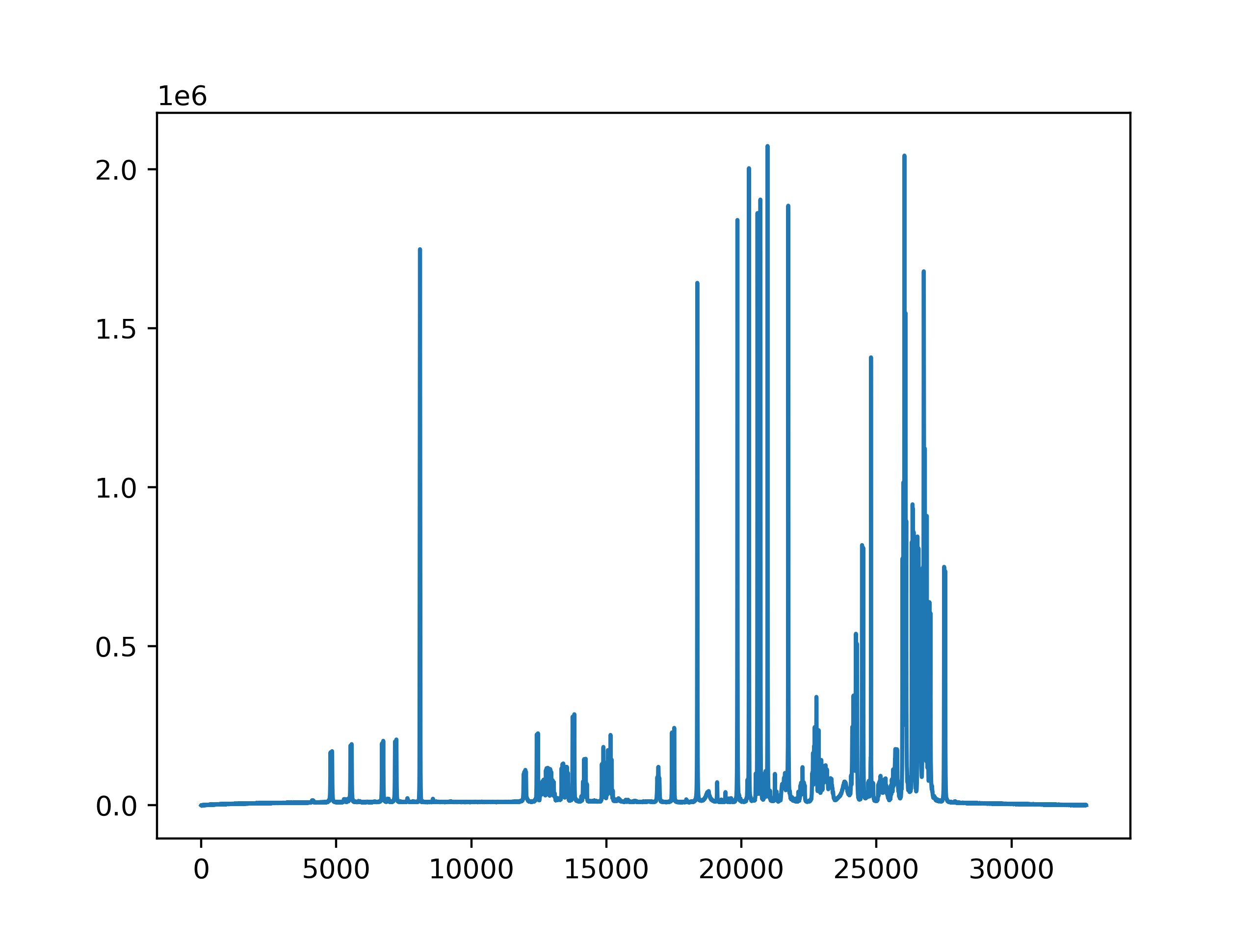
Accessing the Data

I am working with a 1D processed dataset in the following section.

The data can be obtained in NumPy format, using the data property:

>>> data = dataset.data
>>> print(data.shape)
(32768,)
>>> import matplotlib.pyplot as plt
>>> plt.plot(data)
[<matplotlib.lines.Line2D object at 0x7fb5aa2c4a90>]
>>> plt.show()

Accessing Chemical Shifts/Timepoints

To obtain chemical shifts for processed data, or timepoints for time-domain data, use the get_samples() method:

>>> import bruker_utils as butils
>>> # 1d time-domain data
...
>>> fid_1d = butils.BrukerDataset('data/1')
>>> fid_1d.get_samples()
[array([0.000000e+00, 1.820000e-04, 3.640000e-04, ..., 5.949398e+00,
       5.949580e+00, 5.949762e+00])]
>>> # 1d processed data
...
>>> pdata_1d = butils.BrukerDataset('data/1/pdata/1')
>>> pdata.get_samples(meshgrid=False)
>>> pdata_1d.get_samples()
[array([ 9.99027508,  9.9899398 ,  9.98960452, ..., -0.99515954,
       -0.99549482, -0.9958301 ])]
>>> # 2d time-domain data
...
>>> fid_2d = butils.BrukerDataset('data/2')
>>> fid_2d.get_samples(meshgrid=False)  # more on meshgrid later...
[array([0.00000e+00, 4.88000e-05, 9.76000e-05, ..., 9.72096e-02,
       9.72584e-02, 9.73072e-02]), array([0.       , 0.0001966,
       0.0003932, ..., 0.024575 , 0.0247716, 0.0249682])]
>>> # 2d processed data
...
>>> pdata_2d = butils.BrukerDataset('data/2/pdata/1')
>>> pdata_2d.get_samples(meshgrid=False)
[array([154.23232066, 154.15272382, 154.07312698, ...,  -8.54322199,
        -8.62281884,  -8.70241568]), array([ 9.66018073,  9.65023914,
        9.64029755, ..., -0.49018526, -0.50012685, -0.51006844])]

The meshgrid argument for N-dimensional data takes the samples for each dimension and creates N-dimensional grids to create co-ordinate matrices. This is very useful when it comes to plotting multidimensional signals. Note that by default this is set to True.

Advice for Plotting Data

Plotting nice figures of NMR data is very simple with the help of bruker_utils, if you are familiar with matplotlib. Below are some examples for inspiration.

You will have to install matplotlib separately for these examples. Running python -m pip install matplotlib should suffice.

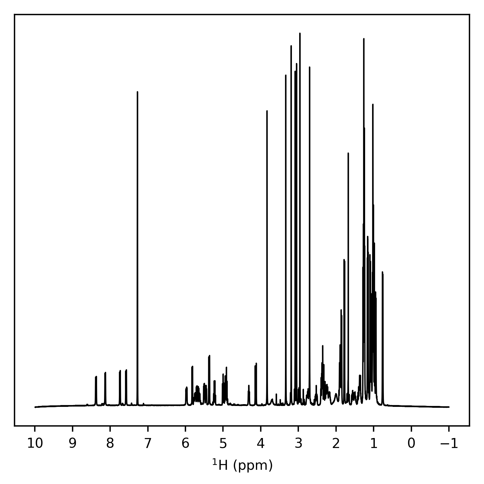
1D Example

Lets write a script which will import 1D processed data, and plot it against its chemical shifts. Key features to note in this script are:

• The spectrum is simply obtained using the data property.

• The shifts are acquired using the get_samples() method.

• As the NMR convention of having chemical shifts go from high to low from left to right is in conflict with the convention of matplotlib to go from low to high from left to right, we need to manually reverse the axis limits (Line 26).

from bruker_utils import BrukerDataset
import matplotlib as mpl
import matplotlib.pyplot as plt


# Make font smaller
font = {'size': 8}
mpl.rc('font', **font)

dataset = BrukerDataset('data/1/pdata/1')
spectrum = dataset.data
# Note that get_samples always returns a list, even
# for 1D data, so we need to unpack it.
shifts = dataset.get_samples()[0]

# Create a figure and axes
fig = plt.figure(figsize=(4, 4))
# list elements are figure co-ordinates for:
# [left, bottom, width, height]
ax = fig.add_axes([0.03, 0.12, 0.94, 0.85])

line = ax.plot(shifts, spectrum, color='k', lw=0.8)
# The x-axis is set to be scending going from left to right
# which is the opposite to NMR convention!
# We need to flip it:
ax.set_xlim(reversed(ax.get_xlim()))
ax.set_xlabel('$^{1}$H (ppm)')

ax.set_xticks(range(10, -2, -1))
# Don't normally show values along the y-axis
ax.set_yticks([])

# Save the figure to your preferred format
fig.savefig('spectrum_1d.png', dpi=400)

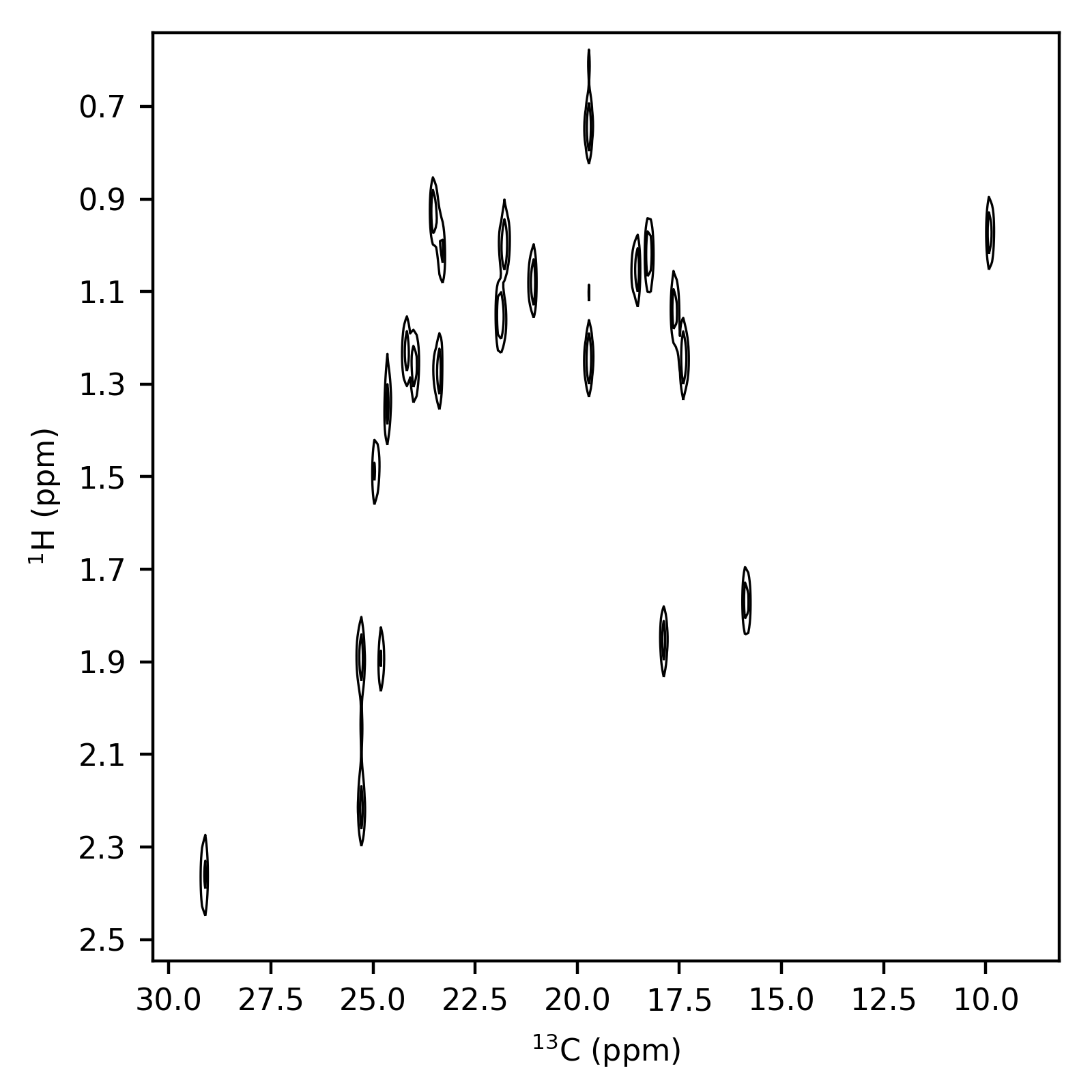
2D Example

Now for an example of a contour for a two-dimensional experiment. Key features here:

• By using get_samples() with meshgrid set to True (default), the shifts is already in the form required for plotting. It simply needs to be unpacked as the first argument in ax.contour (Line 33).

• A list of contour levels is stored with this dataset in the file data/2/pdata/1/clevels. These can be obtained using the contours property (Line 24).

• In this example, this nuclei in each dimension were determined from the NUC1 parameters in acqus and acqu2s. These are denoted as <{number}{symbol}>, where number is the isotope mass number, and symbol is the element symbol. The format_nucleus function is then used to extract the isotope mass and symbol using a regular expression, leading to nicely-formatted axis labels.

import re
from bruker_utils import BrukerDataset
import matplotlib as mpl
import matplotlib.pyplot as plt


def format_nucleus(nucleus: str) -> str:
    """Format nucleus for matplotlib."""
    match = re.search(r'^<(\d+)([A-Z]+)>$', nucleus)
    number = match.group(1)
    symbol = match.group(2)
    return f'$^{{{number}}}${symbol}'


# Make font smaller
font = {'size': 8}
mpl.rc('font', **font)

# Extract spectrum, chemical shifts, and contour levels
# from the dataset
dataset = BrukerDataset('data/2/pdata/1')
spectrum = dataset.data
shifts = dataset.get_samples()
levels = dataset.contours

# Create a figure and axes
fig = plt.figure(figsize=(4, 4))
# list elements are figure co-ordinates for:
# [left, bottom, width, height]
ax = fig.add_axes([0.14, 0.12, 0.83, 0.85])

# Make a contour plot of the spectrum
contour = ax.contour(*shifts, spectrum, levels=levels, colors='k',
                     linewidths=0.6)

# Set x- and y-limit to select the region of interest.
# Note that in each case the order of arguments is (high, low)
# to ensure the axes are flipped.
ax.set_xlim(30.39, 8.2)
ax.set_ylim(2.546, 0.541)

ax.set_xticks([x / 10 for x in range(300, 75, -25)])
ax.set_yticks([x / 10 for x in range(25, 5, -2)])


# Labels for axes.
# This snippet shows how it can be done in an automated fashion
# by extracting the `NUC1` parameter from each acquisition file.
# Also see `format_nucleus` above.
params = dataset.get_parameters(filenames=['acqus', 'acqu2s'])
xnuc = params['acqus']['NUC1']
ynuc = params['acqu2s']['NUC1']
ax.set_xlabel(f'{format_nucleus(xnuc)} (ppm)')
ax.set_ylabel(f'{format_nucleus(ynuc)} (ppm)')

# Save the figure to your preferred format
fig.savefig('spectrum_2d.png', dpi=400)